The Achilles’ Heel of LLM Inference Performance — Quantizing Activations
Taming the beast of Quantization in Activations
What is Quantization ?

Quantization has its roots in the field of signal processing, where it has been used for decades to convert continuous analog signals into discrete digital representations. In the context of digital communication systems, quantization plays a crucial role in encoding and compressing data for efficient transmission and storage.
In recent years, quantization has gained significant attention in the realm of deep learning and neural networks. As the size and complexity of neural networks have grown exponentially, the computational and memory requirements for training and deploying these models have become increasingly challenging. This has led researchers to explore various techniques to reduce the footprint of neural networks without compromising their performance.
The Need for Quantization in Neural Networks
- Memory Constraints: Modern deep learning models often contain millions or even billions of parameters, requiring substantial memory to store and process. Quantization helps reduce the memory footprint of these models by representing the weights and activations with lower precision, such as 8-bit integers instead of 32-bit floating-point numbers.
- Computational Efficiency: High-precision floating-point operations are computationally expensive, especially on resource-constrained devices like mobile phones or embedded systems. By quantizing the weights and activations, neural networks can leverage integer arithmetic, which is faster and more efficient than floating-point operations.
- Energy Efficiency: The energy consumption of neural network inference is directly related to the amount of data movement and computation required. Quantization reduces the data size and simplifies the computations, leading to lower energy consumption and longer battery life on mobile and edge devices.
- Deployment Challenges: Deploying large neural networks on resource-limited devices poses significant challenges due to memory limitations and processing power constraints. Quantization enables the deployment of complex models on a wider range of devices by reducing their memory footprint and computational requirements.
Quantizations Methods
Quantization-Aware Training (QAT)
Quantization-Aware Training (QAT) is a technique where quantization is simulated during the training process, allowing the model to learn to handle reduced-precision representations of weights and activations. Unlike post-training quantization, which applies quantization only after the model has been fully trained, QAT introduces quantization effects while the model parameters are still being optimized. This approach typically yields higher accuracy after quantization, as the model adapts to work with quantized representations from the outset.
How QAT Works
During QAT, simulated quantization steps are inserted into the training pipeline. For example:
- Weight Quantization: Weights are quantized to lower precision (e.g., 8-bit integers) during the forward pass, but the backpropagation algorithm continues to use high-precision floating-point values to update the weights. This approach preserves gradient accuracy.
- Activation Quantization: Activations are also quantized during training. QAT simulates reduced-precision activation values by quantizing them in each forward pass. This step allows the model to “learn” how to work with quantized activation values, reducing the impact of quantization on model performance.
Benefits of QAT
- Higher Accuracy: Since the model learns to compensate for quantization errors during training, QAT typically results in better accuracy than post-training quantization.
- Flexibility in Precision Control: QAT supports mixed-precision approaches where specific layers are quantized to different bit widths based on sensitivity. For example, more critical layers can be quantized with higher precision to minimize accuracy loss.
Challenges of QAT
- Resource Intensity: QAT requires significant computational resources during training due to the need to simulate quantization while maintaining gradient precision.
- Training Complexity: Implementing QAT requires careful management of quantization scaling factors and bit widths, particularly for activations where distributional shifts can heavily impact performance.
Post-Training Quantization (PTQ)
Post-Training Quantization (PTQ) is an efficient quantization approach applied to a model after it has been fully trained. PTQ transforms the trained floating-point model into a quantized version by mapping weights and, optionally, activations to lower precision, typically without any additional training. This approach is quick and resource-efficient, making it popular for models where minor accuracy loss is acceptable in exchange for faster and more compact deployment.
Types of Post-Training Quantization
- Weight-Only Quantization: In this variant, only the model’s weights are quantized to a lower precision, while activations remain in floating-point precision. This technique provides model compression and some latency reduction without heavily affecting accuracy.
- Dynamic Range Quantization: In dynamic range quantization, both weights and activations are quantized, but activation quantization occurs only during inference. This technique doesn’t require any changes to the model architecture or training, making it an accessible option for post-training quantization.
- Full Integer Quantization: Both weights and activations are quantized to integer values for maximum compression and efficiency. This technique typically requires representative data to compute the optimal range for activation quantization, as distributional shifts can otherwise introduce accuracy degradation.
Benefits of PTQ
- Efficiency: PTQ is computationally efficient, as it bypasses the need for additional training. It can be applied to pre-trained models and deployed almost immediately.
- Compatibility with Existing Models: PTQ can be applied to any pre-trained model without modifying the original training pipeline, making it adaptable and flexible.
Within these two main types, we can have:
- Weight-Only Quantization: Only the weights are quantized.
- Activation-Aware Weight Quantization: Weights are quantized with consideration of the distribution of activations.
- Activation and Weight Quantization: Both weights and activations are quantized, offering maximum compression but with greater complexity.

Quantizing Weight vs Activations
Quantizing weights is easier than quantizing activations because weights remain constant during inference, while activations change dynamically based on the input. This static nature of weights allows for a simpler quantization process, as the optimal quantization parameters can be determined offline and applied consistently during inference. Quantizing activations, on the other hand, requires real-time quantization during inference, which is more challenging due to the dynamic range and distribution of activation values. Additionally, the impact of quantization errors on activations can propagate through the network, potentially leading to more significant accuracy degradation compared to weight quantization. Therefore, weight quantization is often preferred as a more straightforward approach to reduce model size in LLMs.
Weight-only quantization enables smaller models and faster latency, but with 16-bit activations, the compute runs through the same 16-bit tensor cores as the unquantized model. This leads to slower inference for compute-heavy workloads due to the penalty of dequantizing the weights.
Weight-only quantization often fails to deliver speed improvements in production serving deployments. These environments typically result in compute-bound workloads with minimal benefits from weight-only quantization. Activation quantization, however, offers a substantial performance boost in such high-compute scenarios and faster inference at lower queries per second (QPS).

Quantization Challenges with LLMs
Quantizing large language models (LLMs) is crucial for reducing their computational footprint and enabling deployment on resource-constrained hardware. However, several challenges arise in attempting to quantize these models effectively, especially transformer-based models like BERT. This section explores the key challenges of quantization, how these challenges were identified, and their underlying causes.
One of the primary challenges in quantizing LLMs is the presence of high dynamic activation ranges within the residual connections. Transformers, especially in deeper layers, exhibit a substantial variability in the range of activation values across different data sequences. This variability becomes a bottleneck when applying quantization, particularly with low-bit formats (e.g., 8-bit), leading to information loss and performance degradation. Residual connections are integral to transformer architectures, allowing the network to mitigate vanishing gradients and improve model convergence. However, in quantized models, the outputs from residual connections exhibit a high variance, leading to significant difficulties in representing the activations accurately with low-bit fixed-point numbers.

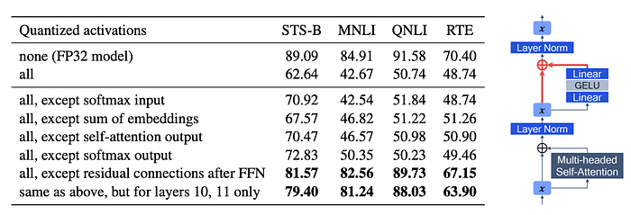
The paper “Understanding and Overcoming the Challenges of Efficient Transformer Quantization” , does a systematic study on the effect of activations in the BERT based architectures to find the regions in the network that lead to performance degradation.he authors of the paper investigated quantization challenges by applying 8-bit post-training quantization to the BERT model and evaluated its performance on various downstream tasks from the GLUE benchmark. The quantization used standard uniform affine quantization with symmetric weight quantization and asymmetric activation quantization.
The performance results indicated that joint 8-bit quantization (for both weights and activations) caused a significant degradation across multiple GLUE tasks. This degradation was much more pronounced compared to when only weights or only activations were quantized. To pinpoint which parts of the network were causing the most issues, an ablation study was conducted where individual components of the transformer (e.g., self-attention outputs, sum of embeddings, etc.) were selectively excluded from quantization. The results of this ablation study were summarized in Table 2, where the performance metrics improved significantly when residual connections after the feed-forward network (FFN) were excluded from quantization.

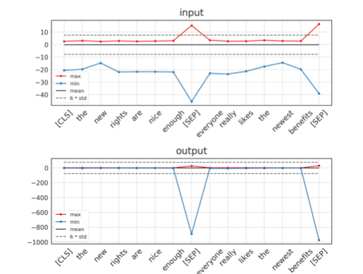
Above plot provides a detailed look into the input and output activation ranges within the 11th layer of BERT. The plots show the substantial difference between the input and output activation ranges of the FFN. The input and output activations had radically different dynamic ranges, with strong outliers being present in the output activation tensor
The primary reason behind this challenge is the mismatch between the activation ranges in residual connections. Residual connections involve adding the input of a layer to its output, which often leads to compounded differences in magnitude. When these activation ranges differ significantly, representing them using a uniform quantization scheme becomes very challenging.
Let’s understand above with an example. Consider the 11th layer of BERT, where the input to the FFN has a relatively narrower range compared to the output, which includes large outliers. This substantial difference can be observed in Figure 2a, where the y-axis scales for input and output activations vary widely. During quantization, if the entire dynamic range of the FFN’s output is considered, it leads to very coarse quantization of the input activations, resulting in quantization errors. Conversely, focusing on preserving higher precision for the input leads to aggressive clipping of the output range, which in turn loses critical information.
How activation function acts as magnitude boosting catalyst ?
The Gaussian Error Linear Unit (GELU) activation function can make the output activation values larger because of the way it handles both positive and negative inputs with a non-linear curve.

where P(X ≤ x) is the cumulative distribution function (CDF) of a standard Gaussian distribution.
In simpler terms, GELU selectively scales inputs based on their values. It behaves differently for negative, small, and large positive values.
- Positive inputs close to or greater than 0 tend to pass through the GELU almost unchanged because the Gaussian CDFapproaches 1 for these inputs. This leads to large positive outputs similar to the input values.
- Negative and smaller positive inputs are reduced in magnitude, as the CDF is much less than 1 for these values, resulting in smaller output values.
This selective behavior of GELU leads to a broader output range, particularly with large positive values remaining largely unaffected, while smaller and negative values are reduced. This broad output range contributes to the high dynamic activation range, which makes quantization challenging.
Consistent Scaling Factor Across Input and Output: When a singular quantization scheme is used, both the input and output activations are quantized using the same range and scaling factor. This means that, regardless of the difference in dynamic range between input and output, the quantization step sizeis identical for both. When these quantized values are added in a residual connection, they are already in the same representation space — making the arithmetic operation straightforward and consistent.
GLU Variants in the FFN Layer
Another activation function to be seen causing problems with activation is GLU unit in the Llama breed models. It is present in the FFN layer of the network. It is similar problem pointed out in the above GELU case leading to activation spikes for specific tokens.
- Layer-Specific Occurrence: Activation spikes predominantly occur in specific layers of the model, particularly in the early and late layers of the FFN.
- Token-Specific Spikes: These spikes are associated with specific tokens rather than being uniformly distributed across a sequence.
There are two techniques mentioned in the paper that helps evade the problem of activation spikes.
- Quantization-free Module (QFeM): This approach involves selectively excluding certain linear layers from quantization, particularly those where large quantization errors are observed. By assessing the extent of scale disparity, QFeM identifies and isolates problematic layers to prevent performance degradation.
- Quantization-free Prefix (QFeP): QFeP focuses on identifying prefixes in the input sequence that trigger activation spikes. By preserving the context of these prefixes as key-value (KV) caches, QFeP prevents the recurrence of activation spikes in subsequent tokens.
The authors conducted extensive experiments on modern LLMs incorporating GLU variants, including LLaMA-2/3, Mistral, Mixtral, SOLAR, and Gemma. The results demonstrate that the proposed methods effectively enhance activation quantization performance, especially when using coarse-grained schemes. Notably, these methods improve upon current techniques like SmoothQuant, which struggle to manage activation spikes.
The Mystery of Activation Spikes: Why Special Tokens Cause a Stir
In the world of LLMs, where billions of parameters work together to understand and generate human language, there’s a peculiar phenomenon that’s been causing a bit of a headache for researchers: activation spikes. These spikes are unexpectedly large activation values that pop up in certain layers of the LLM, particularly in those that use a component called a GLU (Gated Linear Unit). And intriguingly, they seem to be particularly fond of special tokens like the BOS (beginning-of-sentence) token.
But why do these special tokens, like the humble BOS, cause such a stir in the LLM’s activations? The sources offer some clues, suggesting a complex interplay of factors:
- GLUs: The Usual Suspects: The sources strongly implicate GLU variants in the generation of activation spikes. These architectural components, specifically the “down” modules within the FFN (feed-forward network), seem to have a knack for producing these outsized activation values.
- Special Roles for Special Tokens: The BOS token isn’t just any token; it marks the very beginning of a sequence, signaling the start of a new linguistic journey for the LLM. The sources suggest that LLMs might be designed to assign particular importance to certain tokens, and the BOS token, given its unique role, could be receiving special treatment. This emphasis might lead to the amplification of its activations in specific layers.
- Hidden Connections: The sources point to a correlation between activation spikes and the appearance of large-scale values in the intermediate hidden states of the LLM. This suggests that the FFN, through its calculations and the way it integrates information through residual connections, could be playing a part in boosting those hidden state magnitudes, potentially setting the stage for activation spikes to emerge.
- A Dynamic Dance: Adding to the puzzle, the sources note that activation spikes aren’t a constant companion to the BOS token. Their occurrence is dynamic, influenced by the specific context of the input sequence. This means that the surrounding tokens and the LLM’s internal state at any given moment seem to play a role in determining whether the BOS token will trigger a spike.
While the sources provide a fascinating glimpse into the potential reasons behind the BOS token’s spiky behavior, the exact mechanisms remain an open question. Further research is needed to fully unravel the interplay between token characteristics, LLM architecture, and sequence context that gives rise to activation spikes.
Summary of Challenges in Quantizing LLMs
Quantizing large language models (LLMs) introduces significant challenges, particularly due to the presence of activation spikes and high dynamic activation ranges. These challenges are compounded by the structure of transformer architectures, where specific layers and connections are especially sensitive to quantization errors. Both papers identify that outliers in activation values — commonly referred to as activation spikes — cause significant quantization bottlenecks. These spikes are often context-dependent and can vary across different layers and input tokens, leading to non-uniform challenges throughout the model.
One major challenge is the high variability in activation ranges, particularly in residual connections. These residuals can have highly different ranges for input and output activations, complicating their representation using low-bit quantization formats. This mismatch can result in substantial quantization errors when attempting to add quantized values in a residual connection, leading to performance degradation.
Another key issue is that certain layers or modules are inherently more sensitive to quantization, particularly those with high max-median activation ratios, which are indicative of activation spikes. These layers contribute disproportionately to overall quantization errors, making them quantization bottlenecks. To mitigate these issues, the explained papers propose selective quantization or quantization-free approaches for layers with high activation spikes, emphasizing the importance of careful calibration to identify problematic layers and adapt the quantization process accordingly.
Experiment and Results: Benchmarking Llama 3.1–8B Model Performance on A100 80GB GPU
In our experiment, we benchmarked the Llama 3.1–8B model across three configurations: Vanilla (FP16), Weight-Only Quantization (W-INT8-A-FP16 using bitsandbytes), and Weight and Activation Quantization (W-INT8-A-INT8 using NeuralMagic + vLLM). The model was deployed on an A100 PCIe 80GB single GPU instance, using different batch sizes ranging from 1 to 512. We measured three key metrics: Time to First Token (TTFT), Inter-Token Latency (ITL), and Throughput. All other generation parameters, including input prompt, max output tokens, and temperature, were held constant to isolate the effect of batch size on performance.
Time to First Token (TTFT)

The TTFT metric indicates how quickly the model starts generating tokens after receiving an input prompt, providing a view into initial response latency. Across the configurations, we observed the following:
- Vanilla Model: The TTFT remained relatively low and consistent for smaller batch sizes, but we see a rise as the batch size increases, especially beyond 128, indicating potential resource strain.
- Weight-Only Quantization: This configuration showed consistently higher TTFT across all batch sizes, suggesting that the quantized model with FP16 activations incurs a significant overhead during the first token generation. This may be due to the additional computational requirements of dequantizing weights and recalculating activations at the start of each response.
- Weight and Activation Quantization: This configuration consistently achieved the lowest TTFT across batch sizes. This suggests that full quantization (W-INT8-A-INT8) can lead to faster initial token generation by reducing the computational load compared to the vanilla model and weight-only quantization.
For applications where latency for initial response is critical (e.g., interactive applications or customer-facing chatbots), the W-INT8-A-INT8 configuration demonstrates significant advantages, enabling faster response times without sacrificing resource efficiency.
Inter-Token Latency (ITL)

The ITL metric reflects the latency between successive tokens, which directly impacts the speed and fluency of response generation for larger outputs.
- Vanilla Model: ITL was steady at smaller batch sizes but increased progressively at larger sizes, showing potential inefficiencies in scaling with batch size.
- Weight-Only Quantization: The ITL was considerably higher than that of the vanilla model, indicating that quantization, in this case, introduces delays between token generation steps, likely due to handling mixed precision operations.
- Weight and Activation Quantization: This configuration consistently exhibited the lowest ITL across batch sizes, particularly for larger ones, where it demonstrated up to a 60% reduction in latency compared to the vanilla model. This suggests that fully quantized models can improve token processing speed, likely by reducing memory transfer demands and using fewer floating-point operations.
For generating long, uninterrupted responses (e.g., document generation or language translation), weight and activation quantization proves advantageous. Reduced ITL in the W-INT8-A-INT8 configuration can significantly enhance user experience by providing more fluid and responsive outputs.
Throughput

Throughput measures the number of tokens generated per second and is crucial for high-throughput scenarios, such as batch processing or large-scale content generation.
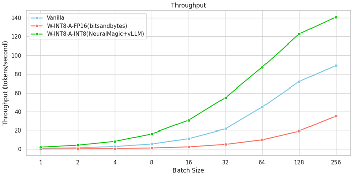
- Vanilla Model: Throughput scaled with batch size up to a point but leveled off beyond batch size 128, indicating resource saturation.
- Weight-Only Quantization: Throughput was consistently lower than the vanilla model across all batch sizes, likely due to the overhead from mixed precision operations.
- Weight and Activation Quantization: This configuration achieved the highest throughput across all batch sizes, peaking at 142 tokens/second at batch size 512. The W-INT8-A-INT8 model’s superior efficiency at large batch sizes makes it highly suitable for processing high volumes of content in parallel.
For applications requiring maximum throughput (e.g., batch content generation, data labeling, or training data augmentation), W-INT8-A-INT8 provides clear benefits. By leveraging full quantization, organizations can achieve greater processing efficiency, particularly when handling large-scale workloads on limited GPU resources.
Takeaways and Future Considerations
The results from this benchmarking study provide several actionable insights for deploying large language models in production:
- Prioritize Full Quantization for Low-Latency Applications: For scenarios where response speed is crucial, such as real-time chat or customer support, using W-INT8-A-INT8 configuration allows for quicker responses with lower latency, without the cost overhead of using a vanilla model.
- Optimize Throughput for Batch Processing Needs: Applications like large-scale document processing, summarization, or data generation would benefit from the W-INT8-A-INT8 configuration, particularly at high batch sizes. The improved throughput enables faster processing and scalability, making it a cost-effective choice for intensive workloads.
- Batch Size Trade-offs: While increasing batch size can improve throughput, it also increases TTFT and ITL due to hardware saturation. For tasks sensitive to initial response time, keeping the batch size under 64 may offer a good balance between efficiency and speed.
- Deployment Flexibility with Quantization: The choice between weight-only and full quantization should be informed by the specific application needs. Weight-only quantization may still be suitable for tasks where memory constraints are paramount, but it may incur higher latency. Full quantization, on the other hand, is ideal for applications that require both high speed and efficient scaling.
- Evaluate GPU Resource Allocation: Given the A100 80GB GPU’s capacity, future optimizations could consider distributing workloads across multiple GPUs or incorporating adaptive batch sizing, where batch size dynamically adjusts based on system load.
Closing note : Accurate benchmarking is indispensable for organizations seeking to deploy LLMs efficiently. It enables an understanding of how each configuration will perform in specific applications, guiding decisions on model and hardware selection. Regular benchmarking is also crucial as models, hardware, and optimization techniques continue to evolve, ensuring that deployment strategies remain effective and cost-efficient over time. While activation quantization offers substantial performance advantages, it also introduces challenges that need careful management. With thoughtful benchmarking and a deep understanding of quantization trade-offs, organizations can harness the full power of large language models, achieving both efficiency and scalability across diverse applications.
References
- https://neuralmagic.com/blog/llm-compressor-is-here-faster-inference-with-vllm/
- Gray, R. M., & Neuhoff, D. L. (1998). Quantization. IEEE transactions on information theory, 44(6), 2325–2383.
- Gersho, A., & Gray, R. M. (2012). Vector quantization and signal compression (Vol. 159). Springer Science & Business Media.
- Cheng, Y., Wang, D., Zhou, P., & Zhang, T. (2017). A survey of model compression and acceleration for deep neural networks. arXiv preprint arXiv:1710.09282.
- Gholami, A., Kim, S., Dong, Z., Yao, Z., Mahoney, M. W., & Keutzer, K. (2021). A survey of quantization methods for efficient neural network inference. arXiv preprint arXiv:2103.13630.
- Han, S., Mao, H., & Dally, W. J. (2015). Deep compression: Compressing deep neural networks with pruning, trained quantization and huffman coding. arXiv preprint arXiv:1510.00149.
- Krishnamoorthi, R. (2018). Quantizing deep convolutional networks for efficient inference: A whitepaper. arXiv preprint arXiv:1806.08342.
- Mitigating Quantization Errors Due to Activation Spikes in GLU-Based LLMs
- Outlier Dimensions that Disrupt Transformers are Driven by Frequency
